Neural Networks

COMPARISON AMONG BACKPROPAGATION LEARNING METHODS

Abstract: This paper analyzes and compares several improvements to the backpropagation method for weights adjustments for a feed-forward network. Therefore, the networks’ behavior is simulated on six certain specific applications. It is also presented a method using a variable step and its superiority is proved by simulation.
1.Introduction Any feed-forward network has a layer-like structure. Each layer is made up of units which receive inputs from the immediate-preceding units and send their outputs to the very next following units. 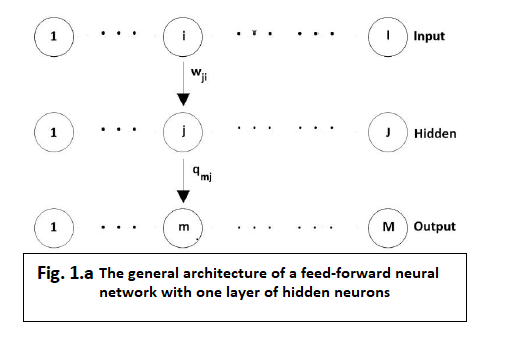The rule that gives the synaptic weights is called the backpropagation rule. Albeit it is possible, it is not necessary to apply this rule to more than one hidden units layer because it has been shown [3] that a single hidden units layer is enough to approximate by a certain precision any function with a finite number of discontinuities if the hidden units are being activated by non-linear functions. Most of the time, applications use a feed-forward network with one hidden units layer and the sigmoidal function to activate the units.For a typical 3-layer network(figure 1.a) the network state is given by the following equations:

$y_{m}=\mathfrak{F}(a_{_m});\textrm{&space;}a_{_m}=\sum_{j=1}^{J}q_{mj}\cdot v_{j}-s_{m},\textrm{&space;}m=\overline{1,M}\textrm{&space;}(1)$ $v_{j}=\mathfrak{F}(\overline{a_{j}});\textrm{ }a_{j}=\sum_{i=1}^{I}w_{ji}\cdot x_{i}-c_{j},\textrm{ }j=\overline{1,J}\textrm{ }(2)$

The synaptic weights (w_ji and q_mj ) and the bias potentials ( s_m and c_j) have to be selected so that the total error:

$\mathbf{J_{s}}(\mathbf{ W,Q,s,c})=\sum_{\mu }^{ } J__{s}^{\mu }$

Is as small as possible. $J_{s}^{\mu }$ is the square error at the output of pattern μ:
$\mathbf{J_{s}^{\mu}}=\frac{1}{2}\cdot \sum_{m=1}^{M}\left [ d_{m}^{\mu }-\mathfrak{F(a_{m}^{\mu })} \right ]^{2} (4)$

where d^μ is the desired output array for class μ. It can be seen that the back-propagation rule is a generalization of the delta rule. Accordingly, we have to calculate the gradient of J, in relation to each parameter and then to modify proportional with this gradient the values of the corresponding parameter. In the first place, we consider only the synaptic connections of the output neurons:
$\Delta q_{mj}= -\rho \cdot \frac{\partial J_{s}}{\partial q_{mj}}=-\rho \cdot \sum_{\mu}^{ }\frac{\partial J_{s}^{\mu }}{\partial q_{mj}}\cdot \frac{\partial a_{m}^{\mu }}{\partial q_{mj}} =\rho \cdot \sum_{\mu}^{ }[d_{m}^{\mu }-\mathfrak{F(a_{m}^{\mu })}]\cdot \mathfrak{F(a_{m}^{\mu })}\cdot \frac{\partial a_{m}^{\mu }}{\partial q_{mj}}\equiv \rho \cdot \sum_{\mu}^{ }\Delta _{m}^{\mu \cdot V_{j}^{\mu }} (5))$

In the next step, we consider the parameters associated to the synaptic connections between the input layer and the hidden one. The procedure is alike, only it needs two substitutions: $\Delta S_{m}= -\rho \cdot \frac{\partial J_{s}}{\partial J_{m}}=\rho \cdot \sum_{\mu}^{ }[d_{m}^{\mu }-\mathfrak{F(a_{m}^{\mu })}]\cdot \mathfrak{F(a_{m}^{\mu })}\cdot \frac{\partial a_{m}^{\mu }}{\partial S_{m}}=- \rho \cdot \sum_{\mu}^{ }\Delta _{m}^{\mu }= \rho \cdot \sum_{\mu}^{ }\Delta _{m}^{\mu }\cdot (-1)$ $\small \Delta _{m}^{\mu }=[d_{m}^{\mu }-\mathfrak{F(a_{m}^{\mu })}]\cdot \mathfrak{F(a_{m}^{\mu })} (7)$ $\Delta w_{ji}=-\rho \cdot \frac{\partial J_{s}}{\partial w_{ji}}=-\rho \cdot \sum_{\mu }^{ }\sum_{m=1}^{M}\frac{\partial J_{s}^{\mu }}{\partial a_{m}^{\mu }}\cdot \frac{{\partial a_{m}^{\mu }}}{\partial v_{j}}\cdot \frac{\partial v_{j}}{\partial w_{ji}}=\rho \cdot \sum_{\mu }^{ }\sum_{m=1}^{M}[d_{m}^{\mu }-\mathfrak{F(a_{m}^{\mu })}]\cdot \mathfrak{F(a_{m}^{\mu })}\cdot\frac{{\partial a_{m}^{\mu }}}{\partial v_{j}}\cdot \frac{\partial v_{j}}{\partial w_{ji}}=\rho \cdot \sum_{\mu }^{ }\sum_{m=1}^{M}\Delta _{m}^{\mu }\cdot q_{mj}\cdot \mathfrak{F}(\overline{a_{J}^{\mu }})\cdot \frac{\partial\overline{ a_{J}}}{\partial w_{ji}}\equiv \rho \cdot \sum_{\mu }^{ } \overline{\Delta _{J}^{\mu }}\cdot x_{i}^{\mu } (8)$ $\Delta c_{j}=-\rho \cdot \frac{\partial J_{s} }{\partial c_{j}}\equiv -\rho\cdot \sum_{\mu }^{ }\overline{\Delta _{J}^{\mu }}= \rho\cdot \sum_{\mu }^{ }\overline{\Delta _{J}^{\mu }}\cdot (-1) (9)$

where:

$\overline{\Delta _{J}^{\mu }}=\left [ \sum_{m}^{ }\Delta _{m}^{\mu }\cdot q_{mj} \right ]\cdot \mathfrak{F(\overline{a_{j}^{\mu }})}(10)$

It is notable that the synaptic weights adjustment equations (8) and (9) resemble to the synaptic equations (5) and (6), with the difference between $\overline{\Delta _{J}^{\mu }}$ diferă de $\Delta _{m}^{\mu }$ , where from it can be recursively obtained.

The backpropagations method has been also extended to the recurrent networks [11, 12, 13], which became more popular ever since.

The error correction scheme works as if the data referring to the deviation from the desired output would propagate backward through the network, “against the flow” of the synaptic connections. It is doubtable, although not entirely impossible, that such a procedure could be accomplished by the biological neural networks. What’s for certain, is that the backward error propagation algorithm is most appropriate for the electronic computers, in both hardware and software implementations. Recently, a backpropagation-like rule, which is based not on the total mean square error minimization but on the Kullbach data maximization, has been out forward for consideration [2].
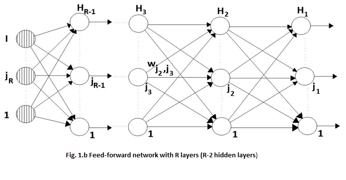The architecture shown in figure 1.a., as good as the relationships (5) – (10), can be extended to a R-layers feed-forward network (R-2 hidden units layers), resulting the architecture shown in figure 1.b. The error criterion that has to be minimized is still the square mean error computed for all the training examples set:
$J=\sum_{\mu }{ }\sum_{j_{1}}^{H_{1}}(d_{j_{1}}^{\mu }-v_{j_{1}}^{\mu })^{2} (11)$

The network’s output will be just the output of the last neural layer: $v _{j_{c}}^{\mu }=\mathfrak{F}\left ( \sum_{j_{c+1}=1}^{H_{c+1}} w_{j_{c},j_{c+1}}\cdot v _{j_{c+1}}^{\mu }-s_{j_{c}} \right )(12)$

Using the backpropagation rule, the following relationships will be generated:

$\Delta w_{j_{c},j_{c+1}}=\sum_{\mu }^{ }\Delta_{j_{c}}^{\mu } \cdot v _{j_{c+1}}^{\mu }(13)$

$\Delta _{j_{c}}^{\mu }=\left ( \sum_{j_{c-1}=1}^{H_{c-1}}\Delta _{j_{c-1}}\cdot w_{j_{c-1}j_{c}}\right )\cdot \mathfrak{F}\left ( v_{j_{c}}^{\mu } \right )(14)$

$\Delta _{j_{1}}^{\mu }= \sum_{j_{1}=1}^{H_{1}} \left ( d_{j_{1}}^{\mu }-\nu_{j_{1}}^{\mu } \right )\cdot \mathfrak{F}\left ( v_{j_{1}}^{\mu } \right )(15)$

$\Delta s_{j_{c}}=\sum_{\mu }^{ }\Delta_{j_{c}}^{\mu } \cdot (-1)(16)$

Being a method of square mean error minimization, covering the whole training examples’ set, method based on the negative gradient, the backpropagation method suffers from the general deficiencies of the gradient techniques. These deficiencies are, generally two:

The learning rate, ρ, which gives the step value on the gradient direction, has to small enough. This, because the gradient is a local measure and if ρ is too large, it may happen that the error value J will not decrease but oscillate, and the synaptic coefficients’ array will jump from one edge if the “hole”, where the local minimum is to be found, to the other edge. On the other hand, a too small ρ leads to a too reduced convergence velocity which leads to a too slow learning process. Even if it is possible to determine (with a huge waste of time) a favorable ρ, this optimum modifies itself during the learning process; it also differs from problem to problem.
Unimportant how rapidly the minimum is reached, this will be the nearest local minimum and it will be unable to exit because, being a gradient method, the backpropagation method exploits the local properties of the criterion function. Moreover, it seems that, the larger the searching space (the weights space) dimension is (i.e. we have a larger amount of neurons in the hidden layers), the larger the number of local minimums and, consequently, the “chance” of failing in one of these.

Having insight these perspectives, we shall compare the classic backpropagation method to some improvements mentioned in the literature and, finally we are going to propose a method which converges more quickly and which is able to escape out of the local minimum.
Therefore, we shall simulate the behavior of those networks in solving six typical problems.

2.Problems for which the BP methods had been tested

For each problem it will be specified the number of inputs, outputs and hidden units. In finding out the number of hidden units contained by the hidden layer, it counts the results of other simulations[17], where it is established the fact that, in order to solve the classification problems, it is proper that this number should be closely equal with the arithmetic mean from the number of the input neurons and the number of the output ones, but no less than 10.
2.1. BINAR

This problem consists in determining the parity of a binary 8-bit word (EXCLUSIVE-OR Task) [6, 9].
The network being used will possess therefore 8 input units and one output unit which will be 0 for an even number of “1” bits contained in the word and 1 otherwise. The number of hidden units is 10.
In this problem we chose the network training over the entire set of possible examples, i.e. over 256 examples.

2.2. COUNTER

We intended to design a counter, which counts the number of “1” bits in a binary 4-bit word [6, 9]. So, we shall have 4 input neurons and 5 output neurons, and the output array belonging to the set {(1,0,0,0,0)^T , (0,1,0,0,0)^T, (0,0,1,0,0)^T, (0,0,0,1,0)^T, (0,0,0,0,1)^T} will be equal with the array i (i=1,…,5)if the input array has i-1 “1” bits. The chosen number of hidden units is 10. We trained the networks for all possible training examples; accordingly, this number of possible examples is 2⁴=16.
2.3. MULTIPLEXOR

The neural network that will simulate the multiplexor will have to learn to assign to the 3-bit input array (3 input neurons) (b₁, b₂, b₃)^T at the output , the 8-bit array(0,..0,1,0,..,0) with only one “1” bit at position i= b₁•2²+b₂•2+b₃. The training examples number is 2³=8 [6], and the number of hidden units is, obviously, also equal with 10.

2.4. 5x5 TABLE

This problem is the problem pertaining to recognizing (classifying) rows and columns into a binary figure. The image is represented by 5×5 (5 rows and 5 columns, i.e. 25 input units, accordingly 25 of input neurons). Due to the fact that each image may contain the same number of rows and columns, we shall need 2 output neurons; the number of neurons from the hidden layer was chosen equal with 14.
Considering the image given by the matrix C [n,m], (n,m=1,…,5), then the input arrays x[i] will be formed by taking i=3∙(n-1)+m. We chose the learning simulation for a set of 16 examples, for each of them giving, as in every supervised leaning process, also the desired output array d:

x d
11111.00000.00000.00000.00000 1 0
00000.11111.00000.00000.00000 1 0
00000.00000.11111.00000.00000 1 0
00000.00000.00000.11111.00000 1 0
00000.00000.00000.00000.11111 1 0
10000.10000.10000.10000.10000 0 1
01000.01000.01000.01000.01000 0 1
00100.00100.00100.00100.00100 0 1
00010.00010.00010.00010.00010 0 1
00001.00001.00001.00001.00001 0 1
11111.11111.00000.00000.00000 1 0
00000.00000.00000.11111.11111 1 0
11000.11000.11000.11000.11000 0 1
00011.00011.00011.00011.00011 0 1
10000.01000.00100.00010.00001 1/2 1/2
00001.00010.00100.01000.10000 1/2 1/2

2.5. ASSOCIATIVE MEMORY

It is tested the “feature extraction” capability of neural networks, i.e. the possibility of memorizing the input “shapes” in a smaller dimension array. Therefore, the network is trained so that to a 16-bit input array will be assigned at the output the same array (also 16-bit long) [9, 10]. The difficulty consists of the fact that the hidden layer has only 4 neurons. We trained the networks over a set of 16 examples: the arrays with the i-th component equal with 1 (i=1,…,16) and the remaining components equal with 0.

2.6. FUNCTION

Beyond the recurrent networks (able to represent time series) in process emulation are also used the feedforward networks, connected as shown in the architecture in figure 2.a. [14,15].

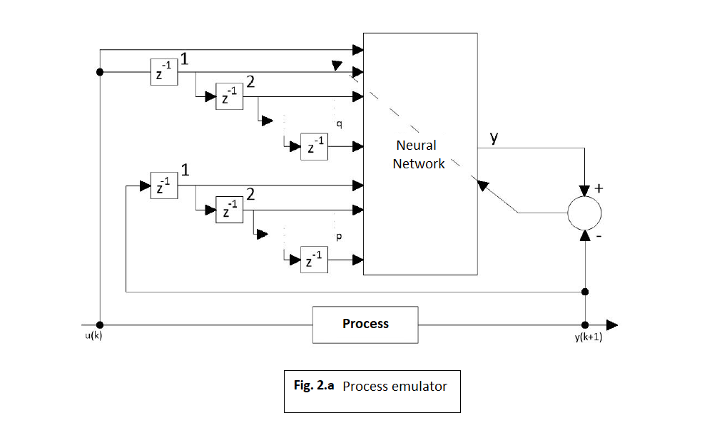
Given p and q, a process can be emulated with a neural network with m-p+q+1 inputs and one output. Writing the representation given by the emulator as φ_E( •) and its output with y’ we have:

$y'=\varphi_{E} (X_{E})(17)$

where:

$x_{E}(k)=[y(k),y(k-1),...,y(k-p+1),u(k),u(k-1),...,u(k-q)]^{T}(18)$

The emulator is trained to minimize the emulating error value: y(k+1)-y’. in figure 2.a., z^(-1) means the delay operator.
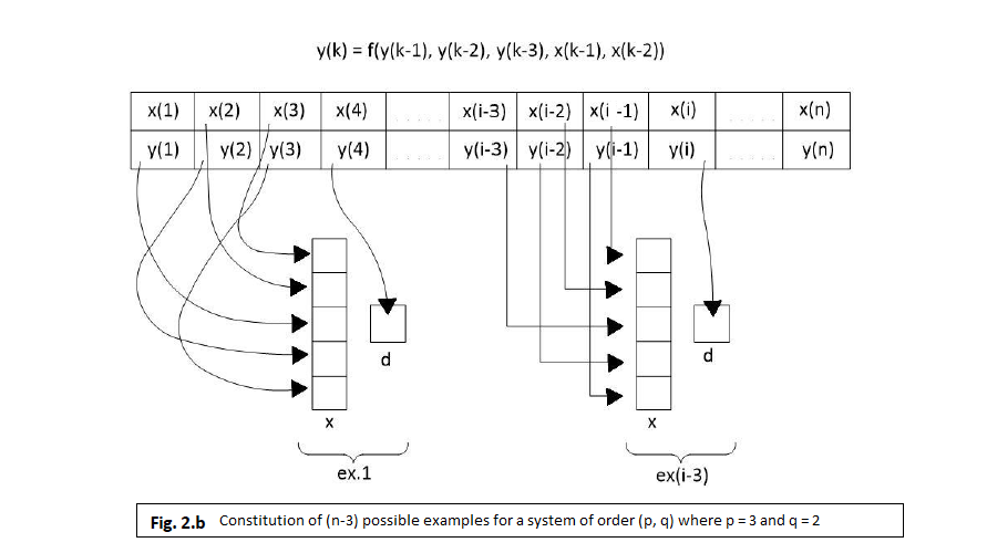
For testing the learning methods, we chose a 2-grade operator. Deeply non-linear, which has been used in [5] and which is being taken from [8]. The system is described by the equation:

$y(k)=\frac{y(k-1)\cdot y(k-2)\cdot [y(k-1)+2,5]}{1+y^{2}(k-1)+y^{2}(k-2)}+u(k)(19)$

where u(k) is a sinusoidal signal:

$u(k)=sin(0,08\cdot \pi \cdot k)(20)$

We generated 80 pairs (u(k), y(k)) starting from y(-1)=0 and y(0)=1 and we used them for the off-line networks training.
As the general procedure stipulates, we presumed to be known the SISO process rank (Signal Input Single Output) and, thereby, we chose a network with 3 input units, an output unit and 10 hidden units. The input units are connected as shown in figure 2.b. in the following way: at moment k, the three x units will be jointed one of each to y(k-2), y(k-1) and u(k), while the desired output, d, will be considered y(k). Actually, since the output of any neuron is always between 0 and 1, we have to proceed to a conversion of y’s value in this interval. We chose a linear transforming method of the definition domain for y in the interval (0.15, 0.85) to allow the network to adapt also to signals which beyond the learning period would quit the training values’ boundaries. Hence, we compute the mean Medy for y’s values over the training set and then, MaxDy which is the absolute value of the values’ deviation from the computed mean, which leads to the following:

$d(k)=\frac{1}{2}+0,7\cdot \frac{|y(k)-Medy|}{MaxDy}(21)$

Different from other authors, we don’t follow a likewise operate for inputs: such an operation would probably soften the adapting process, but it would complicate the training architecture because it would have to distinguish between input types (which yield from the process’s inputs and which from its outputs).
3. LEARNING METHODS
3.1. BackPropagation Classic (BP)
The classic method allows the user to choose the learning rate, i.e. the step value towards the criterion function gradient J. as shown in paragraph 1, this value shouldn’t be too large nor to small. Up until now, there hasn’t been brought up any general method for choosing ρ for a given problem. It is recommended that ρ should be smaller than 1 or, eventually decreasing with the growth of the iteration number.
It has been shown that the decreasing velocity of the criterion function strongly depends on the chosen value for ρ. Generally speaking, it is recommended to test the network evolution for a several values of ρ and then to pick up a suitable value. One could start by taking a relative small values for ρ and then increasing this value, as long as this decreases J. When ρ exceeds the optimum and becomes too large, oscillations of J’s values will appear, which sometimes grow larger instead if diminishing.
We tested the network behavior for several ρ values, choosing the optimum.
However, it is not only ρ that is unknown, as it may seem at first sight, but also the initial settings for the network weights. These are being randomly chosen within [-1,1]. Lastly, it would be wrong to choose ρ for a certain set of weights. That is why we simulate each network behavior, for each ρ, for 10 problems, whatever the learning method and the variable parameters are, we consider each time the same 10 sets if initial random weights.
Each method was run the same amount of time. Because the iterations do not last equally, even for the same method, we also represented on the abscissa on figure 3 the running time (2 minutes on a PC-IBM 486; 50 MHz; but this is unimportant fir the methods comparison).
On the ordinate, we represented the decimal logarithm of the criterion function J for the whole examples set. We preferred the logarithmic representation for the reason that errors each anyway much smaller values than the initial ones, but their ranking at different moments of time counts.
Each line containing 3 graphics presents, briefly, the simulation’s results for a certain problem. The left graphic presents $lg \underset{i=1,10}{\underline{max}}J_{i}(t;\rho )$ ,where i is the i-th set of initial weights for a given ρ at any moment t of time. The right graphic is presents the $lg \underset{i=1,10}{\underline{max}}J_{i}(t;\rho )$ functions, and the middle one is $\lg \left [ \frac{1}{10}\cdot \sum_{i=1}^{10}J_{i}(t;\rho ) \right ]$ , hence it refers to the criterion functions mean for a certain ρ.

In order to select the most favorable value for ρ we compare the logarithm means curves (the middle graphic), and in the case of several values with close results we will also consider the other graphics. For the reason of graphic unambiguity, we haven’t sketched the curves for all values of ρ for which we simulated the network behavior.
The following simulations had been made:
1).BINAR: ρ=0.1 (curves 1); ρ=0.18; ρ=0.26 (curves 2); ρ=0.3; ρ=0.34 (curves 3);
ρ=0.38; ρ=0.42 (curves 4); ρ=0.5.
The best result: ρ=0.34 (curves 3).
2).COUNTER: ρ=0.1; ρ=0.18 (curves 1); ρ=0.26; ρ=0.34 (curves 2); ρ=0.42; ρ=0.5 (curves 3); ρ=0.58; ρ=0.66 (curves 4).
The best result: ρ=0.5 (curves 3).
3).MULTIPLEXOR: ρ=0.1; ρ=0.18; ρ=0.26; ρ=0.34; ρ=0.42 (curves 1); ρ=0.5; ρ=0.58; ρ=0.66 (curves 2); ρ=0.74; ρ=0.82; ρ=0.9 (curves 3); ρ=0,98; ρ=1.06; ρ=1.14; ρ=1.22 (curves 4); ρ=1.3.
The best result: ρ=1.22 (curves 4).
4).5×5 TABLE: ρ=0.1 (curves 1); ρ=0.18 (curves 2); ρ=0.26; ρ=0.34 (curves 3); ρ=0.42; ρ=0.5; ρ=0.58 (curves 4); ρ=0.66.
The best result: ρ=0.58 (curves 4).
5).ASSOCIATIVE MEMORY: ρ=0.1 (curves 1); ρ=0.18 (curves 2); ρ=0.26; ρ=0.34; (curves 3); ρ=0.42; ρ=0.5 (curves 4); ρ=0.58.
The best result: ρ=0.5 (curves 4).
6).FUNCTION: ρ=0.01 (curves 1); ρ=0.02 (curves 2); ρ=0.04; ρ=0.06 (curves 3); ρ=0.1; (curves 4); ρ=0.18.
The best result: ρ=0.02 (curves 2).

3.2. BackPropagation with Termen Proportion (BPTP)
Because, generally, the convergence is slow for the backpropagation rule, different improvements for the weights adjustment algorithm have been suggested. For the backpropagation algorithm, the learning procedure needs a weights modification proportional to $\frac{ \partial J_{s}^{\mu} }{\partial w}$ .
The negative gradient method impelled infinitesimal steps, the proportionality constant being the learning rate, ρ. For practical reasons, of swifter convergence we select a learning rate as large as possible, without reaching oscillations.
A way for avoiding oscillations at large values for ρ is to alter the weight considering the preceding modification, by adding a proportion term:

$\Delta w_{ji}(k+1)=\rho \cdot \Delta _{j}^{\mu}\cdot x_{i}^{\mu }+\beta \cdot \Delta w_{ji}(k))(22)$
Where k is the iteration number and β is a non-negative constant.
In literature it is asserted that by adding the proportion term, the minimum is more rapid reached because larger learning rates are allowed, without reaching oscillations, it is also recommended that [7] β=ρ/k.

3.3 BackPropagation with Termen Proportion and Restart (BPTPR)

In order to ensure the BPTP algorithm’s convergence, we took β=ρ/k and, after a large number of iterations, β becomes so small that the proportion term has no further contribution in restart, meaning the periodic „restarting” of the weights modifying direction to the gradient direction. Thus:

$\beta _{k}=\left\{\begin{matrix} \rho /i \: \: pentru \: i\neq 0\\0\: \: \: \; \: \: pentru \: i=0 \end{matrix}\right.\; \; unde i=k\: mod\: I\; (23)$

For I=1, this yields in the BPTP method. It is recommended that I should take values between 2 and 10.

This time we have two variables: ρ and i. Considering that the proper value of ρ doesn’t chance too much than in the previous method, we search for the most favorable value of I, holdingρ=ρ_{optimum BPTP} for each problem, and after that, we hold I settled, checking the optimum ρ around the value ρ=ρ_{optimum BPTP}.

3.4. Conjugate Gradient BackPropagation (CGBP)

Another idea was the applying of profound techniques in optimization theory. Actually, it is obvious that BPTPR is a simplified variant of the conjugate gradient with restart method. This method differs from BPTPR only by the selection of β, which here is computed more complicated, according to the gradient norm from the present iteration, k, and from the preceding iteration, k-1, using the following formula:
$\beta _{k}=\left\{\begin{matrix} \frac{g_{i}}{g_{i-1}}\cdot \frac{g_{i}-g_{i-1}}{g_{i-1}}\; for \: i\neq 0\\ 0 \; \;\; \; \; \; \; \; \; \; \; \; \; \; \; \; \; for \: i=0 \end{matrix}\right. unde\; i - k\: mod \: I\: \; (24)$
However, this method also requests to select the coefficient ρ and the restart index i. Therefore, we rerun the simulations in order maintain constant the values of ρ and i. At the beginning we maintain constant value of ρ (ρ_{optimum BPTPR}) and we search for most favourable value of I around I_{optimum BPTPR}. The we hold still I at I_{optimum CGBP}and search for ρ_{optimum CGBP} around ρ_{optimum BPTPR.}
The following simulations have been made (figure 4):
1).BINAR: ρ_BPTPR=0.42 and I=5 (curves 1); ρ_BPTPR=0.42 and I_BPTPR= 6; ρ_BPTPR=0.42 and I=7;
ρ_BPTPR=0.42 and I=8 (curves 2);
ρ_BPTPR=0.42 and I=9; ρ_BPTPR=0.42 and I=10; ρ_BPTPR=0.42 and I=11 (curves 3);
I=11 and ρ=0.34; I=11 and ρ=0.5 (curves 4).
The best result: ρ=0.42 and I=11 (curves 3)
2).COUNTER: ρ_BPTPR=0.42 and I=3 (curves 1);
ρ_BPTPR=0.42 and I_BPTPR=4 (curves 2);
ρ_BPTPR=0.42 and I=5 (curves 3);
ρ_BPTPR=0.42 and I=6; ρ_BPTPR=0.42 and I=7; I=4 and ρ=0.5 (curves 4);
I=4 and ρ=0.58.
The best result: ρ=0.5 and I=4 (curves 4).
3).MULTIPLEXOR: ρ_BPTPR=0.98 and I=4 (curves 1);
ρ_BPTPR=0.98 and I=5 (curves 2);
ρ_BPTPR=0.98 and I=6 (curves 3);
I=5 and ρ=1.06; I=5 and ρ=1.14; I=5 and ρ=1.22; I=5 and ρ=1.3 (curves 4);
I=5 and ρ=1.38.
The best result: ρ=1.3 and I=5 (curves 4).
4).5×5 TABLE: ρ_BPTPR=0.74 and I=2 (curves 1);
ρ_BPTPR=0.74 and I=3 (curves 2);
ρ_BPTPR=0.74 and I=4 (curves 3);
ρ_BPTPR=0.74 and I_BPTPR=5; ρ_BPTPR=0.74 and I=6; I=3 and ρ=0.66; I=3 and ρ=0.82 (curves 4).
The best result: ρ=0.74 and I=3 (curves 2).
5).ASSOCIATIVE MEMORY: ρ_BPTPR=0.42 and I=4; ρ_BPTPR=0.42 and I=5 (curves 1);
ρ_BPTPR=0.42 and I=6; ρ_BPTPR=0.42 and I=7 (curves 2);
ρ_BPTPR=0.42 and I=8; ρ_BPTPR=0.42 and I=9; ρ_BPTPR=0.42 and I=10(curves 3);
ρ_BPTPR=0.42 and I=11; I=10 and ρ=0.34; I=11 and ρ=0.5 (curves 4).
The best result: ρ=0.42 and I=10 (curves 3).
6).FUNCTION: ρ_BPTPR=0.02 and I=2 (curves 1);
ρ_BPTPR=0.02 and I_BPTPR=3; I=2 and ρ=0.06; I=2 and ρ=0.1 (curves 2);
I=2 and ρ=0.18; ρ=0.1 and I=3 (curves 3);
ρ=0.1 and I=4; ρ=0.1 and I=5; ρ=0.1 and I=6 (curves 4); ρ=0.1 and I=7.
The best result: ρ=0.1 and I=6 (curves 4).

Remark: : Comparing the results obtained with the different favorable learning methods among these 4 methods we can see in figure 5 (curve 1: BP; curve 2: BPTP; curve 3: BPTPR; curve 4: CGBP) the detached superiority of the CGBP method. The situation that sometimes came upon (for example, in the COUNTER problem) where, though for some initial weights we gain quite satisfying results, sometimes the results are weaker than those obtained with other methods, is due to the following two reasons:
a) The high computing complexity implies for the same running time less learning iterations being executed;
b) Maybe the running time has been too little for the decreasing tendency of the CGBP algorithm getting to lower the criterion function at smaller values.

3.5. BP and CGBP using the error’s absolute value minimization criterion

In all hereby presented examples, the weights had been computed in terms of the mean square error. The following problem is put forward: which would be the network behavior if instead of the square error one would consider the absolute output error value? We studied this problem in the case of two learning methods: BP and CGBP, which proved to be the best.
The total error will be computed using the same formula (3), but $J_{s}^{\mu }$ , the absolute output error for pattern μ, will be:

$J_{s}^{\mu }=\frac{1}{2}\cdot \sum_{m=1}^{M}\left | d_{m}^{\mu }- \mathfrak{F}\left ( a_{m}^{\mu } \right ) \right | (25)$
Where, as in the preceding case, d^μ is the desired output array for the class μ.
Following exactly the same reasoning presented widely by the relationships (5)-(10), there will yield the relationships to be applied in this case:

$\Delta q_{mj}=\frac{\rho }{2}\cdot \sum_{\mu }\sigma \left [ d_{m}^{\mu}-\mathfrak{F(a_{m}^{\mu}}) \right ]\cdot\mathfrak{F(a_{m}^{\mu})}\cdot\frac{\partial a_{m}^{\mu}}{\partial q_{mj}}=\frac{\rho }{2}\cdot \sum_{\mu }\Delta _{m}^{\mu }\cdot v_{j}^{\mu } (26)$

$\Delta s_{m}= -\frac{\rho }{2}\sum_{\mu }\Delta _{m}^{\mu } (27)$

$\Delta _{m}^{\mu }=\sigma\left[d_{m}^{\mu}-\mathfrak{F(a_{m}^{\mu}})\right]\cdot\mathfrak{F(a_{m}^{\mu})}(28)$

Where, by σ[expression] we considered the function that return the sign of the given expression.
Likewise, will be done for the parameters assigned to the synaptic connections between the input and the hidden layer:

$\Delta w_{ji}=\frac{\rho }{2}\cdot \sum_{\mu }\overline{\Delta}_{j}^{\mu }\cdot x_{i}^{\mu }(29)$

$\Delta c_{j}=\frac{\rho }{2}\cdot \sum_{\mu }\overline{\Delta }_{j}^{\mu } (30)$

$\overline{\Delta _{J}^{\mu }}=\left [ \sum_{m}^{ }\Delta _{m}^{\mu }\cdot q_{mj} \right ]\cdot \mathfrak{F(\overline{a_{j}^{\mu }})}(10)$

Extending to a feedforward R-layers network, the error criterion that should be minimized is the absolute error value determined over the set of all training examples:

$J_{p}=\frac{1}{2}\cdot \sum_{\mu }\sum_{j_{1}=1}^{H_{1}}\left | d_{j_{1}}^{\mu }-v_{j_{1}}^{\mu } \right | (32)$

The expression (13-16) can be easily altered for the present case; the major modification is linked to the formula (15) which becomes:

$\Delta _{j_{1}}^{\mu }=\sum_{j_{1}=1}^{H_{1}}\sigma \left [ d_{j_{1}}^{\mu }-\nu _{j_{1}}^{\mu } \right ]\cdot \mathfrak{F}\left ( \nu _{j_{1}}^{\mu } \right )(33))$

For the same problems for which the previous learning methods were tested, we have run simulation programs and their results are represented on graphics, together with the corresponding best result obtained in the case of the square error minimization error. Different from the previous simulations, here we used only one set of initial weights and we kept for graphic representation only the best result. This fact does not influence the final conclusions on the efficiency comparison of the two methods: it can be seen, in most cases, the superiority of the method using the square error minimization criterion over the second method.
On each of the 6 graphics (figure 6a-6f), the curves 1 and 2 represent the best result obtained with the BP, accordingly the CGBP method, using the second error minimization criterion, and the curves 3 and 4 represent the best result after applying the same learning methods (BP, acc. CGBP) but for the first error minimization criterion (the square error minimization).

For the BP method (curves 1), we started initially from the most favorable value for ρ, for which we obtained the best network’s behavior as shown in paragraph 3. We varied ρ until the best behavior for the absolute error value criterion has been reached. This is represented by the curves 1 and these must be compared to the curves 3 (BP for the square mean error).

For the CGBP method (curves 2), the initial parameters were: optimum ρ found before and the optimum restart index I_{optimum CGBP,} but using the square error method. The ρ coefficient was kept constant and the index I was varied; then, after choosing an optimum I, this was kept constant and ρ was varied until the most suitable was reached. With these two best parameters, for each application has been represented on graphic, curves 2 which must be compared with curves 4.

The following simulates were run:
1).BINAR: BP: ρ=0.66 (curve 1); CGBP: ρ=0.82, I=11 (curve 2);
BP: ρ=0.34 (curve 3); CGBP: ρ=0.42, I=11 (curve 4).
2).COUNTER: BP: ρ=0.5 (curve 1); CGBP: ρ=0.5, I=4 (curve 2);
BP: ρ=0.5 (curve 3); CGBP: ρ=0.42, I=4 (curve 4).
3).MULTIPLEXOR: BP: ρ=1.22 (curve 1); CGBP: ρ=1.22, I=5 (curve 2);
BP: ρ=1.22 (curve 3); CGBP: ρ=1.3, I=5 (curve 4).
4).5X5 TABLE: BP: ρ=0.58 (curve 1); CGBP: ρ=0.58, I=4 (curve 2);
BP: ρ=0.58 (curve 3); CGBP: ρ=0.74, I=3 (curve 4).
5).ASSOCIATIVE MEMORY: ρ=0.5 (curve 1); CGBP: ρ=0.5, I=10 (curve 2);
BP: ρ=0.5 (curve 3); CGBP: ρ=0.42, I=10 (curve 4).
6).FUNCTION: BP: ρ=0.0005 (curve 1); CGBP: ρ=0.5, I=10 (curve 2);
BP: ρ=0.02 (curve 3); CGBP: ρ=0.1, I=6 (curve 4).

Conclusions
The usual BP methods need testing processes in order to find out the optimum value for ρ, value that depends on the given problem to be learned. The more refined methods also request the determining of I.
Hence, beside the swifter convergence of the proposed method, this has also the advantage of relieving the user from performing preliminary tests to determine ρ and I. It should be noted that the changes made upon simulating programs when passing from one method to another were as small as possible, searching to modify the running times only by enlarging the computing complexity.
Although the neural networks are typical parallel structures, the simulation was accomplished on a computer using a sequential algorithm. In the case of a parallel structure implementation, the comparison should be made not on the same running time, but on the same number of iterations. In such a case the superiority of the proposed NBP method would be increased.

References

Battiti, R. ; Masulli, F. – ”BFGS Optimization for faster and automated supervised learning” – in “Proc. of the ICANN” – Espoo, Finland, June, 1991.
Benaim, M.; Tomasini, L. – “Competitive and self-organizing algorithms based on the minimisation of an information criteria” – in “Artificial Neural Networks”/ Kohonen, T.; Mkisara, K. ; Simula, O. ; Kanga, J.(Ed.) – Elsevier, North-Holland, 1991.
Hornik, K. ; Stinchcombe, M. ; White, H. – “Multiplayer feedforward networks are universal approximators” – Neural Networks, nr.2 – 1989; pp. 359 – 366.
Hou, T. – H.; Lin, L. – “Manufacturing process monitoring using neural networks” – Computers & Elect. Engineering – Vol. 19, No. 2, 1993 – pp. 129 – 141.
Hush, D.; Abdallah, C.; Horne, B. – “The recursive neural network and its applications in control theory” – Computer & Elect. Engineering – Vol. 19, No. 4, 1993 –pp. 333-341.
Jacobs, R.A. – “Increased rates of convergence through learning rate adaptation” – Neural Networks – vol. 1, 1988 – pp. 295-307.
Krse, B.J.A.; Smagt, P.P. van der – “An Introduction to Neural Networks” – The University of Amsterdam, 1993.
Narendra, K.; Parthasarathy, K. – “Identification and control of dynamical systems using neural networks” – IEEE Trans. On Neural Networks – Vol.1, No. 1, 1990 – pp. 4-27.
Ooyen, A. van; Nienhuis, B. – “Improving the convergence of the back-propagation algorithm” – Neural Networks –vol.5, 1992 – pp.465-471.
Philips, S.; Wiles, J. – “Exponential generalization from a polynomial number of examples in a combinatorial domain” – in “Proceedings of the International Joint Conference on Neural Networks: IJCNN’93”- Nagoya, Japan, October 1993, pp. 505-508.
Pineda, F. J. – “Generalization of backpropagation t recurrent and higher order neural networks” – in “Proceedings of IEEE Conference on Neural Information Processing Systems”/Anderson, D.Z. (Ed.) – Denver, CO – November, 1987.
Pineda, F.J. – “Dynamics and architecture for neural computation” – Journal of Complexity – No. 4, 1988 – pp. 216-245.
Pineda, F.J. – “Recurrent backpropagation and the dynamical approach to adaptive neural computation” – Neural Computation – No.1, 1989 – pp.161-172.
Pourboghrat, F. – “Adaptive neural controller design for robots” – Computers & Elect. Engineering – Vol.19, No. 4, 1993 – pp. 277-288.
Ribar, S.; Koruga, D. – “Neural networks controller simulation” – in “Proc. of the ICANN” – Espoo, Finland, June, 1991.
Silva, F.M.; Almeida, L.B. – “Speeding up backpropagation” – in “Advanced neural computers”/Eckmiller, R (Ed.) – North-Holland, 1990 – pp. 151-160.
Volovici, D. – “The reliability of flexible technological processes” (Ph. D. Thesis) – Politehnica University of Bucharest, Faculty of Electronics and Telecommunications, 1994.
Williams, R.J.; Zipser, D. – “A learning algorithm for continually running fully recurrent neural networks” – Neural Computation – No.1; 1989, MIT – pp.270-280.

useful